In 2026’s lecture, Tensor einops was talked at first.
Tensor operations #
Tensor storage #
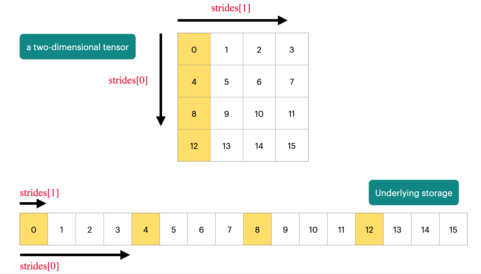
PyTorch tensors are pointers into allocated memory with metadata describing how to get to any element of the tensor.
x = torch.tensor([
    [0., 1, 2, 3],
    [4, 5, 6, 7],
    [8, 9, 10, 11],
    [12, 13, 14, 15],
])

# Go to next row (dim 0), skip 4 elements
assert x.stride(0) == 4
# Go to next column (dim 1), skip 1 element
assert x.stride(1) == 1
# To find a element:
r, c = 1, 2
index = r * x.stride(0) + c * x.stride(1)
assert index == 6
Tensor slicing #
Many operations simply provide a different view of the tensor, which means they do not make a copy.
x = torch.tensor([[1., 2, 3], [4, 5 ,6]])
y = x[0]
assert same_storage(x, y) # not built-in function

y = x[:, 1]
assert same_storage(x, y)

y = x.view(3, 2)
assert same_storage(x, y)

y = x.transpose(1, 0)
assert same_storage(x, y)

x[0][0] = 100
assert y[0] == 100

x = torch.tensor([[1., 2, 3], [4, 5, 6]])
y = x.transpose(1, 0)
assert not y.is_contiguous()
try:
    y.view(2, 3)
    assert False
except RuntimeError as e:
    assert "view size is not compatible with input tensor's size and stride" in str(e)

y = x.transpose(1, 0).contiguous().view(2, 3) # Hard copy happened
assert not same_storage(x, y)
Tensor elementwise #
These operations apply some operations to each elements of the tensor and return a (new) tensor of the same shape.
x = torch.tensor([1, 4, 9])
assert torch.equal(x.pow(2), torch.tensor([1, 16, 81]))
assert torch.equal(x.sqrt(), torch.tensor([1, 2, 3]))
assert torch.equal(x.rsqrt(), torch.tensor([1, 1 / 2, 1 / 3]))  # i -> 1/sqrt(x_i)

assert torch.equal(x + x, torch.tensor([2, 8, 18]))
assert torch.equal(x * 2, torch.tensor([2, 8, 18]))
assert torch.equal(x / 0.5, torch.tensor([2, 8, 18]))
triu takes the upper triangular part of a matrix
x = torch.ones(3, 3).triu()
assert torch.equal(x, torch.tensor([
    [1, 1, 1],
    [0, 1, 1],
    [0, 0, 1,]
]))
Tensor matmul #
x = torch.ones(16, 32)
w = torch.ones(32, 2)
y = x @ w
assert y.size() == torch.Size([16, 2])
In general, we perform operations for every example in a batch and token in a sequence.
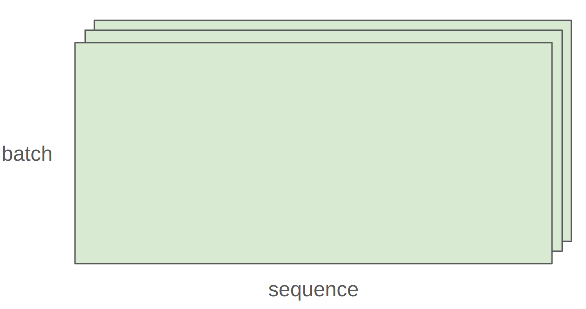
x = torch.ones(4, 8, 16, 32)
w = torch.ones(32, 2)
y = x @ w
assert y.size() == torch.Size([4, 8, 16, 2])
In this case, we iterate over values of the first 2 dimensions of x and multiply by w. (batched matmul + automatic broadcasting)
Tensor einops #
Einops motivation #
In tranditional PyTorch code, it is easy to mess up the dimensions.
Einops is a library for manipulating tensors where dimensions are named. It is inspired by Einstein summation notation (Einstein, 1916). [Einops tutorial]
Jaxtyping basics (from 2025) #
Old way:
x = torch.ones(2, 2, 1, 3) # batch seq heads hiddenNew (jaxtyping) way:
# from jaxtyping import Float
x: Float[torch.Tensor, "batch seq heads hidden"] = torch.ones(2, 2, 1, 3)This is just documentation (no enforcement), which means such code below is legal:
x: Float[torch.Tensor, "batch seq heads hidden"] = torch.ones(100, 5)Einops einsum #
Einsum is generalized matrix multiplication with good bookkeeping.
x: Float[torch.Tensor, "batch seq1 hidden"] = torch.ones(2, 3, 4)
y: Float[torch.Tensor, "batch seq2 hidden"] = torch.ones(2, 3, 4)
Old way:
z = x @ y.transpose(-2, -1) # batch, sequence, sequenceNew (einops) way:
# from einops import einsum
z = einsum(x, y, "batch seq1 hidden, batch seq2 hidden -> batch seq1 seq2")
Or can use ... to represent broadcasting over any number of dimensions:
z = einsum(x, y, "... seq1 hidden, ... seq2 hidden -> ... seq1 seq2")Einops reduce #
You can reduce a single tensor via some operation (e.g., sum, mean, max, min).
x = torch.ones(2, 3, 4)  # batch seq hidden

# Old way
y = x.sum(dim=-1)

# New (einops) way
y = reduce(x, "... hidden -> ...", "sum")
Einops rearrange #
Sometimes, a dimension represents two dimensions, and you want to operate on one of them.
x = torch.ones(3, 8) # seq total_hidden… where total_hidden is a flattened representation fo heads * hidden1 (2x4 matrix)
w = torch.ones(4, 4) # hidden1 hidden2Break up total_hidden into two dimensions (heads and hidden1)
x = rearrange(x, "... (heads hidden1`) -> ... heads hidden1`", heads=2)Perform the transformation by w
x = einsum(x, w, "... hidden1, hidden1 hidden2 -> ... hidden2")Combine heads and hidden2 back together
x = rearrange(x, "... heads hidden2 -> ... (heads hidden2)")Tensor operations flops #
A floating-point operation (FLOP) is a basic operation like addition (x + y) or multiplication (x y).
Intuitions #
Traning GPT-3 (2020) took 3.14e23 FLOPs. Training GPT-4 (2023) is speculated to take 2e25 FLOPs.
H100 has a peak performance of 1979 TFlop/s with sparsity, 50% without [specs]
Linear model #
if torch.cuda.is_available():
    B = 16384  # Number of points
    D = 32768  # Dimension of each point
    K = 8192   # Number of outputs
else:
    B = 1024
    D = 256
    K = 64
x = torch.ones(B, D, device=cuda_if_available())
w = torch.randn(D, K, device=cuda_if_available())
y = x @ w
How many FLOPs is this matmul? We have one multiplication (x[i][j] * w[j][k]) and one addition per (i, j, k) triple.
actual_num_flops = 2 * B * D * K We can also time this operation to see how long it takes.
actual_time = benchmark(lambda: x @ w) The actual FLOP/s of this operation:
actual_flop_per_sec = actual_num_flops / actual_time Each GPU has a specification sheet that provides the peak performance. Note that the FLOP/s depends heavily on the data type!
promised_flop_per_sec = get_promised_flop_per_sec(x.dtype) Model FLOPs utilization (MFU) #
MFU = (actual FLOP/s) / (promised FLOP/s) [ignore communication/overhead] Usually, ≥ 0.5 is quite good.
Summary #
- Matrix multiplications dominate: (2 m n p) FLOPs
- FLOP/s depends on hardware (B200 » H100) and data type (bfloat16 » float32)
- MFU: (actual FLOP/s) / (promised FLOP/s)
Arithmetic intensity #
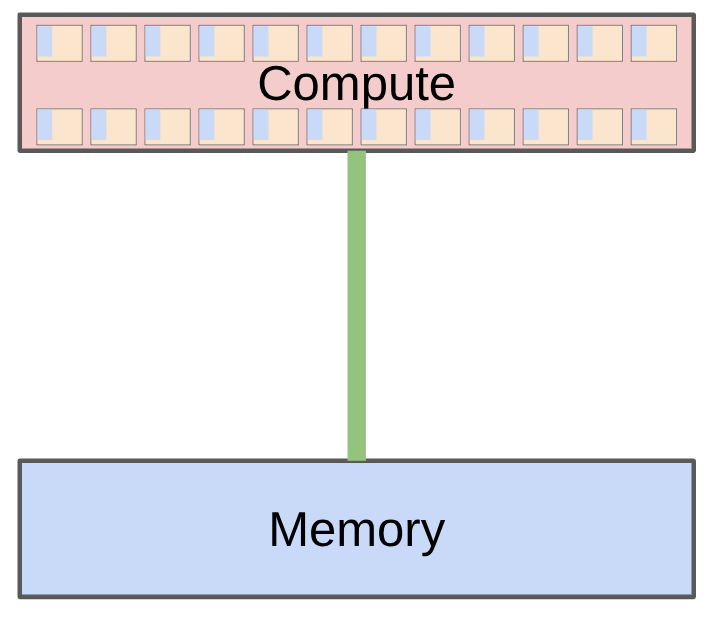
The total time it takes from input to output depends on:
- Accelerator speed (FLOP/s)
- Memory bandwidth (bytes/s)
assert h100_flop_per_sec == 1979e12 / 2  # Half without sparsity
assert h100_bytes_per_sec == 3.35e12
ReLU #
Just in case, $\mathrm{ReLU}(x) = \mathrm{max}(0, x)$
n = 1024 * 1024
x = torch.ones(n, dtype = torch.bfloat16, device = cuda_if_available())
y = torch.relu(x)

bytes = (2 * n) + (2 * n) # Read x, write y (bf16 is 2 bytes/float)
flops = n # n comparisons

communication_time = bytes / h100_bytes_per_sec # 1.252e-6
computation_time = flops / h100_flop_per_sec # 1.060e-9
Arithmetic intensity: how much actual work per byte for this workload?
h100_accelerator_intensity = h100_flop_per_sec / h100_bytes_per_sec # ~295.3731
arithmetic_intensity = flops / bytes # ~1/4
assert arithmetic_intensity < h100_asccelerator_intensity
Apparently, ReLU is memory-bound (commmunication time > computation time), which leads to low MFU.
GELU #
$\mathrm{GELU}(x) = x \cdot \Phi(x) \approx 0.5 x \left( 1 + \tanh \left( \sqrt{\frac{2}{\pi}} (x + 0.044715 x^3) \right) \right)$
In case you forgot, $\Phi(x)$ is cumulative distribution function.
import torch.nn.functional as F

n = 1024 * 1024
x = torch.ones(n, dtype=torch.bfloat16, device=cuda_if_available())
y = F.gelu(x)

bytes = (2 * n) + (2 * n) # Read x, write y (bf16 is 2 bytes/float)
flops = 20 * n

arithmetic_intensity = flops / bytes # ~5
assert arithmetic_intensity < h100_asccelerator_intensity
Obviously GELU has higher arithmetic intensity than ReLU, but it is still memory-bound.
Dot product #
n = 1024 * 1024
x = torch.ones(n, dtype=torch.bfloat16, device=cuda_if_available())
w = torch.ones(n, dtype=torch.bfloat16, device=cuda_if_available())
y = x @ w

bytes = (2 * n) + (2 * n) + 2 # Read x, read w, write y
flops = 2 * n - 1 # n multiplications, n-1 additions

arithmetic_intensity = flops / bytes # ~1/2
assert arithmetic_intensity < h100_asccelerator_intensity
Still memory-bound.
Matrix vector product #
n = 1024
x = torch.ones(n, dtype=torch.bfloat16, device=cuda_if_available())
w = torch.ones(n, n, dtype=torch.bfloat16, device=cuda_if_available())
y = x @ w

bytes = (2 * n) + (2 * n * n) + (2 * n) # Read x, read w, write y
flops = n * (2 * n - 1) # n dot-product

arithmetic_intensity = flops / bytes # ~1
assert arithmetic_intensity < h100_asccelerator_intensity
Memory-bound.
Intensity matmul #
n = 1024
x = torch.ones(n, n, dtype=torch.bfloat16, device=cuda_if_available())
w = torch.ones(n, n, dtype=torch.bfloat16, device=cuda_if_available())
y = x @ w

bytes = (2 * n * n) + (2 * n * n) + (2 * n * n)  # Read x, read w, write y
flops = n * n * (2 * n - 1)  # n^2 dot products

arithmetic_intensity = flops / bytes  # ~n/3
assert arithmetic_intensity > h100_accelerator_intensity # 341.1667 > 295.3731
Obviously, it is compute-bound.
Training Transformers are compute-bound, since it involves big matrix multiplications. Matrix-vector product is what happens during inference, which is why inference is memory-bound.
Arithmetic/accelerator intensity also depends on the precision (bf16 versus fp32)
Roofline plots #
We can visualize the relationship between arithmetic intensity and performance using roofline plots.
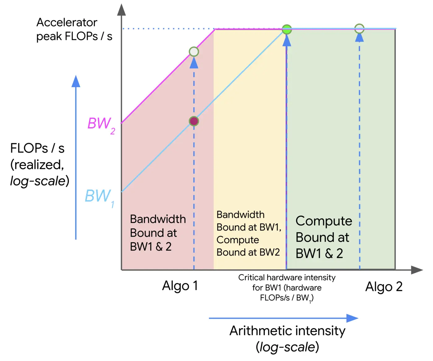
- The red region corresponds to low arithmetic intensity operations (e.g., ReLU, GELU), which are memory-bound — their performance scales with available bandwidth. As bandwidth increases (from BW1 to BW2), performance improves, but only up to a point.
- Once the arithmetic intensity is high enough, the workload enters the yellow zone, where it may be memory-bound under lower bandwidth (BW1) but already compute-bound under higher bandwidth (BW2).
- Finally, in the green region (e.g., matmul), performance is fully compute-bound, and further increases in bandwidth no longer help — only improving compute throughput matters.